Will rapid sea level rise turn our marsh to mud flats and shallow lagoon?
By Peter Vogt, ACLT Founding Member
In the Spring 2021 Newsletter (pg.8), I speculated on the future of the ACLT as the successful land conservancy it has become. Now about the future of the Parkers Creek Preserve (PCP), its dramatic habitat diversity, an island in a vast urban-suburban sea. Our small but growing oasis is protected into the indefinite future for nature and passive human recreation. The protection is by legal, not physical fencing, and how we manage this oasis. Ecology is the response of life to physical forcing—notably climate. Absent human influences, it would be easy to predict the climate, sea level and ecology even millennia from now.
As is, what will happen especially to the salt marsh and adjoining freshwater swamps in the coming decades and centuries is awash in uncertainty. How fast will humans reduce greenhouse gas emissions? How fast and how much will climates change, and how much and how fast will sea levels rise—largely by ice loss in Greenland and Antarctica? How will tidal Parkers Creek and the PCP respond to those distant and global processes? How will PCP biota respond to warmer climates and higher CO2? How much will the oceanic and thus the Chesapeake’s acidity increase, impairing carbonate shell growth by oysters and clams? How much will land-falling tropical cyclones intensify due to a warming Atlantic? Will land-fall frequency change? How might multidecadal variability change—confusing long term climate change predictions?
Instead of using fuzzy terms like ‘the middle of the next century’ I will hazard predictions for four “preservation milestone years.” That’s to sharpen our sense of past and future times, relating the ACLT to older Mid-Atlantic land preserves –all of which still exist today! The Boston Common (A, 1634) was the first urban park; Thomas Jefferson’s sale (B, 1815) of Virginia’s Natural Bridge as a ‘trust’; the oldest land conservancy (Trustees of Preservation, C, 1891); and the first Calvert nature preserve (Hellen Creek hemlocks, The Nature Conservancy, D, 1956). The ACLT is 35 years old this year, and will be as old as A in the year 2373, B in 2192, C in 2116, and D in 2051. While 2373 may feel unimaginably far in the future, that year is actually 35 years closer to us than 1634!
I’ll start by predicting that chemical pollution and its longer lasting effects will continue at least for some decades. Additional alien species will surely invade the PCP. These are biota not yet introduced, plus others, like fire ants, which will migrate up here, enabled by climate warming. If alligators get into Parkers Creek by 2192, would ACLT find them interesting or try to kill them off? Thousand Cankers Disease (fatal to black walnuts) is already in Cecil County, and the spotted lanternfly, chowing down on many tree species, is poised to invade from southeastern Pennsylvania. Insect populations are in decline—which would imperil bats and many of our insectivore song birds. However, future gene editing might safely deal with many pathogens, as it has with the chestnut blight. Given time, native plant species might evolve resistance while some native predators might evolve a taste for invasives.
As the Bay widens by wetland loss in Dorchester County, the increasing fetch would increase Calvert Cliff wave erosion, but warming would also decrease the effect of freeze-thaw. Mostly, climate change and sea level rise won’t have major effects on Calvert Cliffs shoreline retreat rates—see more below.
More frequent high rainfall events will increase slope erosion– but scarcely to high historical erosion rates from farmland. Increasing CO2 will stimulate plant growth (including invasives and poison ivy) but make foliage less nutritious for insects.
Depending on future CO2 (plus other greenhouse gas) emissions, our climate by 2192 and especially 2373 would range from somewhat similar to today to tropical. After that, climates should stabilize and very slowly cool. My optimistic prediction for those distant years is a new Old-Growth forest similar but more bio-diverse than what hikers see today. Some American species will have migrated here from the coastal Carolinas or Georgia. (A pessimist might predict a species-poor environment dominated by invasives, with few trees growing large and old).
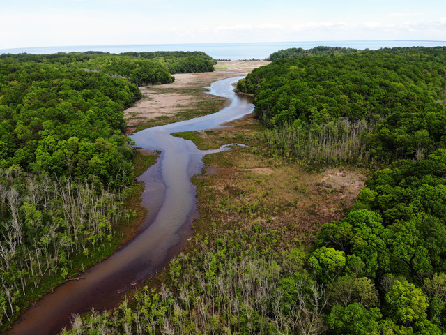
The most dramatic change in the PCP future may well be the transformation- by rapid sea level rise- of the salt marsh and adjacent freshwater swamp. They may turn into mud flats and then a shallow lagoon. A marsh doesn’t care how high sea levels will eventually get—provided the rise is not too rapid.
Sea level rise and land subsidence rates are reported in millimeters per year, where 1 mm/year= 0.39 inches/decade: RSLR means Relative Sea Level Rise, which includes any vertical movement of land, in our area subsidence. RSLR has been measured by tide gauges at some coastal sites for more than a century. Since 1993 it has also been measured by radar pulses reflected from the ocean surface by orbiting earth satellites. Land rise or fall rates are today being measured with GPS. Multi-annual fluctuations (winds, precipitation, etc.) create sea level ‘noise’ which must be smoothed out (filtered) to obtain a time series of sea level versus time. These data are then empirically fit with a simple algebraic function. This function can then be interpolated to get the relative sea level for any given time and place, and used to predict the near-term future.
Future climate change and sea level rise in Maryland have been professionally studied for decades. In 2007 the State established the MD Commission on Climate Change (MCCC), which includes a group of experts. The MCCC regularly issues reports, updating projections, and strategies for mitigation and adaptation. The most recent summary of MD sea level rise was issued in 2018. Projections have become more sophisticated, and are now couched in probability and statistics. For example, Baltimore, having Maryland’s longest tide gauge record, has a 66% probability of RSL being between 0.6 ft and 1.6 ft higher in 2050 than it was in 2000. RSLR has been accelerating at 0.084 mm/year per year—meaning +1.68 mm/year from 2000 to 2020! The prediction for Parker’s Creek would be very slightly higher.
Graphs of future sea level (and other parameters such as global temperature, CO2, and human population) have the alarming, exponential-like shape of explosions. The curves resemble playground slides (if only 1900-2100 is shown), or hockey sticks (if the last 1,000 or 10,000 years are included). Eventually all such parameters will level off or/and decline. The question for humanity—and for the PCP– is what will happen in the interim.
Salt marshes like the one bordering tidal Parker’s Creek grow upwards via new but not decomposing organic matter from plant growth, plus any sediment washed or blown in. Marshes thrive when the RSLR is positive but slow. If RSLR increases too fast, some marshes will just migrate inland, leaving open water in their ‘wakes’. However this is possible only if the land is low and slopes are gentle. The Parker’s Creek marsh and swamp are bordered by relatively high and steep topography, thus preventing migration, i.e., a ‘wetland squeeze’. However, the hilly PCP topography also limits the amount of land flooded by future sea level rise, or land species killed by brackish water, or by shoreline erosion, were the marsh to become a lagoon.
Falling sea levels (caused mainly by ice sheets once again growing) would kill the salt marsh and turn the marsh-swamp of Parkers Creek into forest, somewhat as beaver ponds revert to forest once beavers are gone. However, sea levels won’t fall again for a very long time. Perhaps 15% of the atmospheric CO2 from fossil carbon fuels will stay in the atmosphere for millennia, enough to prevent glacial re-expansion.
What will happen in Parker’s is that the marsh may well not keep up with faster sea level rise, and would essentially drown by flooding. It’s probably not if but when! Scientists will study the process. Whether or not “we” should then artificially maintain the marsh is another matter– for ACLT land managers maybe not yet born.
Salt marshes have become more widespread globally in recent millennia, due to slowing of post-glacial sea level rise. As noted by paleoclimatologist Prof. William Ruddiman, ancient air bubbles trapped in polar ice sheets show that atmospheric methane (CH4) and CO2 began to increase again, respectively around 5000-6000 and 7000-8000 years ago. This did not happen during previous post-glacial times, leading Ruddiman to propose modest but significant pre-Industrial man-made greenhouse gas emission increases. The CO2 increase corresponds to the time of rapid deforestation and farming expansion in Eurasia. The CH4 increase corresponds to expansion of Chinese rice paddy cultivation. The global warming effects of these emissions happened to cancel out a natural 2o C cooling and thus prevented some sea level fall. This implies that many modern salt marshes, including Parker’s, are ultimately due to mankind meddling with climate. (As it happens, Bill Ruddiman is a friend and former coworker, who in the early 70s coincidentally lived in Prince Frederick—in the Parkers Creek watershed).
US Geological Survey cores of Chesapeake Bay area salt marsh burial depths, age-dated by C14 (led by Dr. Tom Cronin of USGS), showed RSLR slowing around 6000 years ago, as the last of the Laurentide ice sheet melted away. This was more than five millennia after climate warming began. It takes time to melt a great ice sheet, and melting mostly occurs only in the warm season. There may have been further slowing to very low RSLR rates around 2000 years ago.
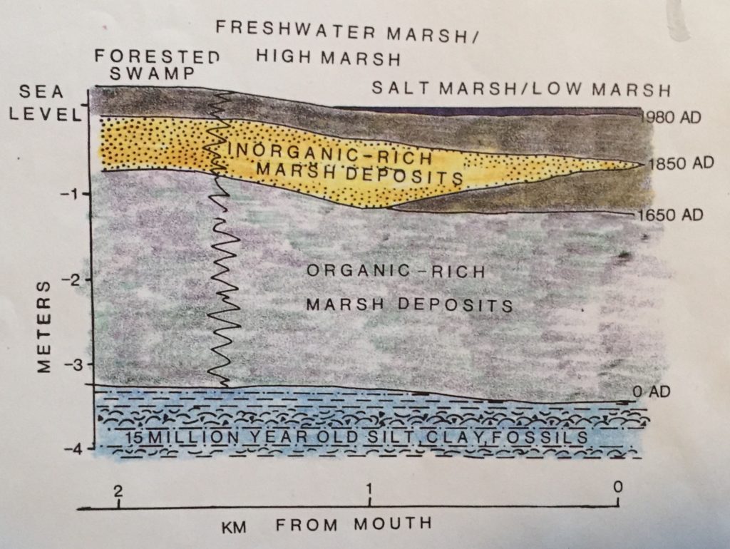
Sediment coring in Parkers marsh by a Johns Hopkins PhD student (Norman Froomer) in the 1970s showed the marsh layer is about 10 ft thick and 2000 years old at its base. The long-term average RSLR has thus been 1.5 mm/year, so the marsh kept up with this slow rise. (I suspect an open lagoon existed for some centuries before, but a barrier beach formed, leading to a marsh protected from Chesapeake waves).
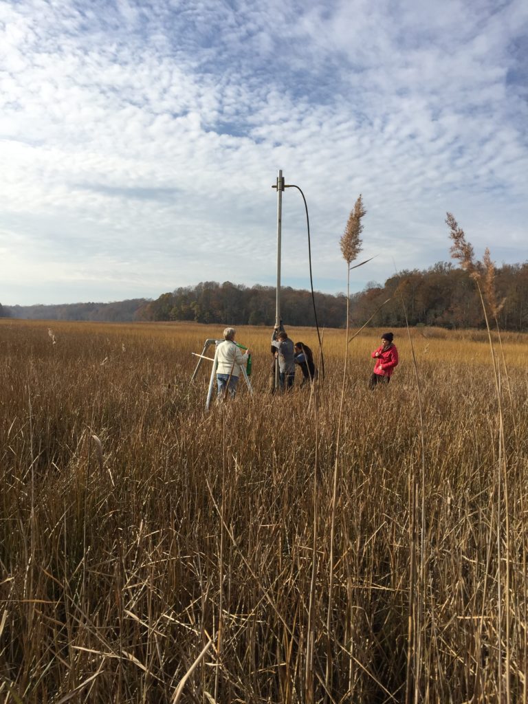
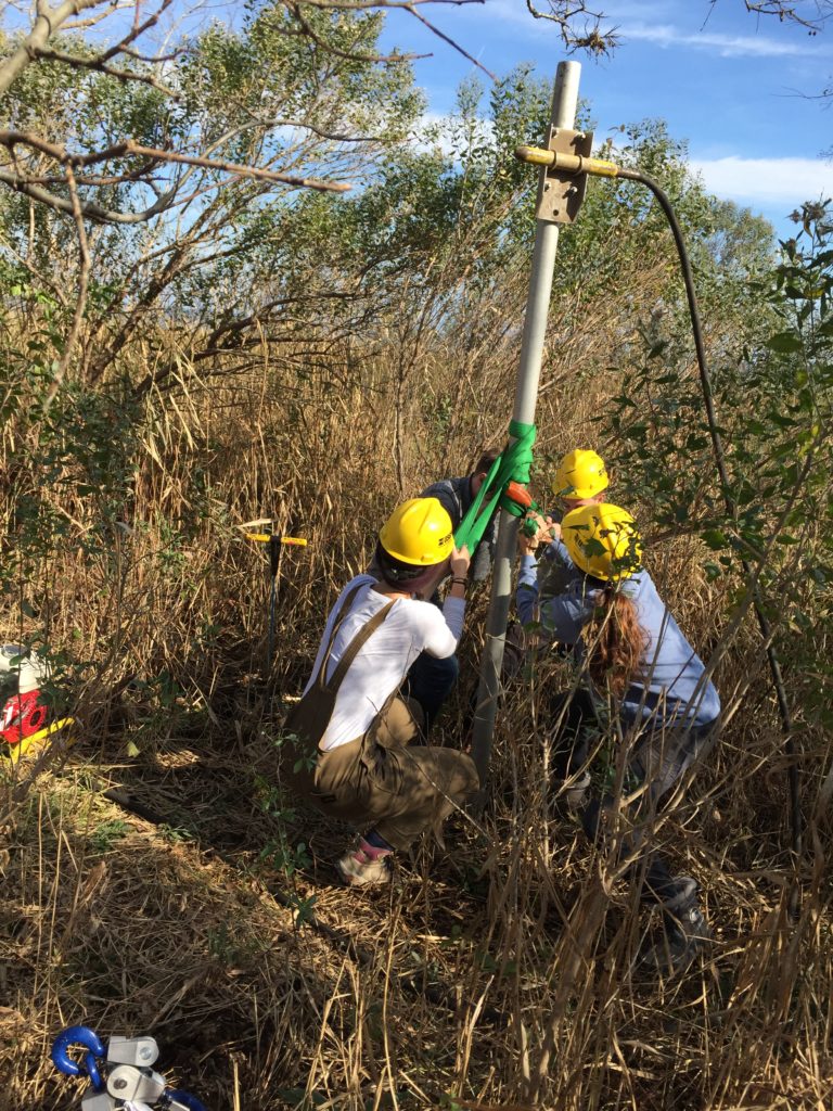
New marsh data are being collected at present. In late 2019, the USGS (Dr. Michael Toomey) took three sediment cores in a short transect from the beach berm inland into the Parker’s marsh. This coring is part of a USGS study to see if marsh sediment piles record long-term storm surge frequency – registered by berm overwash sediment. The Covid-19 pandemic delayed analysis.
In the top 84 cm of the cores, inorganic sediment washed in from the Parker’s watershed records land clearing by early English farmers and their American descendants after the middle 17th century. From this result, Froomer derived an average RSLR of 2.74 mm/year between 1650 and 1975. His other two study marshes, along the tidal Potomac, yielded the same result, but in Parker’s the transition from fresh tidal to brackish had migrated neither towards the Chesapeake (due to sediment input and increased runoff) nor inland (due to sea level rise and westward migration, by shoreline retreat, of the barrier beach). Those 10 ft thick marsh deposits are a priceless archive of past PCP watershed and marsh vegetation, historical land use, and sea level rise. Science has so far barely skimmed this archive.
Meanwhile CBL scientist Dr. Lora Harris and her Lab Assistant Jessica Flester have deployed (2012) four rSETs (rod-surface-elevation tables) in the marsh. The repeated measurements will determine how well the Parker’s salt marsh keeps up with RSLR. The data since 2013-14 offer good news. There is no tide gauge in Parker’s Creek, but Maryland tide gauge data reported in 2018 show RLSR rates since 2000 ranging from 4.2 to 7.3 mm/year. However, Parker’s Creek marsh elevations at the four rSET sites increased even more rapidly (+5.9-+13.9 mm/year), showing the Parker’s marsh (and others in our region) are so far doing well in keeping ahead of the sea level rise. Ironically, the main gas (CO2) that is increasing global sea levels is also encouraging marsh plant growth.
Any change in living marsh vegetation over time and space can record the response to RSLR acceleration, which would increase both salinities and flooding frequency. For example, we predict the Parker’s salt marsh species like Spartina patens (salt hay) will be gradually displaced by the more salt tolerant S. alterniflora (smooth cordgrass). Upstream in the freshwater swamp, narrow-leaf cattail tolerates a bit more brackishness than the common broadleaf cattail. The May 16, 2020 drone image shows some dying trees in the small swamp forests—is this evidence for accelerated sea level rise and increased flooding, or/and increased brackishness? Or was this forest an ‘unnatural’ consequence of greatly increased sediment input from eroding farmland?
According to Dr. Patrick Megonigal of SERC (Smithsonian Environmental Research Center), recent research in the Kirkpatrick salt marsh shows that sedges tolerate more flooding and thrive more under higher CO2 concentrations than do grasses like S. patens. Sedges use a different type of photosynthesis than grasses. Being familiar with the Parker’s marsh, Dr. Megonigal pointed out that our marsh vegetation is already dominated by types of plants like sedge, which should help stabilize our marsh against faster RSLR and extend marsh life by several decades.
How fast is sea level rising today? In recent decades relative sea levels have been rising around 3.5 mm/year in our part of the Chesapeake region, including the PCP. Of that, about 1 mm/year is due to land sinking, the remaining Earth response to the giant Laurentide ice sheet once north of here. Humans can’t change that. Of the remaining 2.5 mm/year, about half has been due to ocean warming and expansion, and the other half to glacier/ice sheet melting adding water to the ocean. Satellite sea level measurements beginning in 1993 plus data from ice sheets suggest that the effect of melting now dominates and has accelerated, with present RSLR likely more like 4.5 mm/year. Limited data from other marshes suggest that the Parker’s salt marsh may not keep up if this rate doubles.
An
additional effect is possible Gulf Stream weakening, an additional RSLR effect
in the Mid-Atlantic. The Gulf Stream circulation ‘holds’ a broad 3 ft high dome
of water centered over the Bermuda region. This is the same Coriolis ‘force’
which also causes the counterclockwise circulation of surface Chesapeake Bay
waters and thus keeps Parkers Creek tidewater less salty than across the Bay.
If the Gulf Stream weakens, the dome height decreases, and water levels rise
here, west of the Gulf Stream. For a salt marsh, even a few inches rapid sea
level rise matters. Increasingly frequent ‘nuisance flooding’ (during normal
high tides) in the Mid-Atlantic may in part reflect Gulf Stream weakening but
is scarcely an issue for a nature preserve.
Long-term (multi-year) natural atmospheric fluctuations—reflected in temperature, winds, or precipitation, and unrelated to climate change—complicate identification of true climate change. One such natural multi-decadal oscillation has a quasi-period of 70-90 years and is generated within overturning of the Atlantic Ocean. This oscillation influences the atmosphere and is recorded as precipitation ‘cycles’ in bald cypress tree rings in the coastal Carolinas and by salinity-sensitive Chesapeake plankton sampled in sediment cores east of Parkers Creek (More watershed precipitation in the Bay watershed means lower Bay salinities). Whether climate change will affect this oscillation—which has been happening for millennia—remains unknown, but both the public and politicians may confuse such long term oscillations with climate change. As two possible local examples, the extreme 2002 drought might easily be blamed on climate change, but occurred 71-73 years after a worse drought (1929-31). In 2002 the freshwater tidal part of Parker’s Creek was brackish for weeks, and upstream of that, the creek turned to isolated mud puddles. How freshwater fish species survived or returned to Parker’s Creek remains a mystery. Some very cold Calvert winters during 1893-1905 were followed more than 80 years later by similar exceptional cold in the late 1970s-early 80s. Yes, I even ice skated on the Chesapeake Bay, Patuxent River, and Parkers Creek! Should we experience unusual cold winters in 2050-60, some might argue that climate warming has ended!
By far the most dramatic water level changes are short term storm surges caused by tropical cyclones-especially for storms tracking northeast with centers west of Parker’s Creek. The amplitude of such surges (roughly + 6 ft during Isabel in 2003) dwarfs the normal tidal range (about 1.46 ft at Parker’s Creek). Surge heights will be greater if Chesapeake shorelines become extensively armored. Future surges will at least add to the expected RSLR, and at worst be more severe if tropical cyclones are strengthened by the warming Atlantic. Future surges will carry brackish water up into parts of Parkers Creek presently upstream of the tides. Whether the PCP fully recovers from future extreme droughts, storm surges and widespread tree blowdowns will test its ecological resiliency.
Different future greenhouse gas emission scenarios give widely different model predictions (2017) of the 2100 increase over 2000 sea levels, from the most optimistic (+ 1 ft) to the most pessimistic (+8.2 ft). The +1 ft prediction is scarcely realizable because it assumed anthropogenic emissions would peak by 2020, which they have not, and that they will decline to zero by 2100. These are the mean global values, and sea level will likely be somewhat higher here. Our 1 mm/year land subsidence adds 4” per century, and any Gulf Stream weakening would add more inches. I will guesstimate +3 ft for the Parker’s Creek area between now and 2116. By 2373 a worst case might be up to +15 ft.
If RSL rises more than ca. ca 6-8 ft in the PCP area, the preserved PCP cliffs south of the Parker’s beach will slow their erosion and shoreline retreat rate (presently around 4”-8”/year) by Chesapeake’s waves, while the PCP cliffs north of the beach will start eroding faster. This gradual switch reflects 1) the tilt (dip) of the Miocene layers (strata) downwards to the southeast and 2) a more erodible layer, the Parkers Creek Bone Bed, currently exposed to wave action south of the beach, will disappear below the waves due to rising RSL. Meanwhile the same layer, currently above the reach of waves further north, will become accessible to wave erosion. Because the barrier beach protecting the salt marsh appears ‘pinned’ to -and thus aligned with- the cliffs, the slow clockwise rotation of the beach and cliffs will change to counterclockwise, and loss of salt marsh behind the beach will switch from greater in the south to greater in the north. These gradual changes are driven by the geology exposed in the cliffs but are speeded up by faster SLR.
Shoreline retreat along the PCP cliffs and the 1300 ft long barrier beach have not been specifically studied. The process can be envisioned as giant horizontal band saw cutting into the shore while gradually being raised. The beach and offshore sand bars migrate inland as they follow the saw. For an assumed ball-park average retreat of 3” per year, the PCP 7700 ft long shoreline will have migrated respectively 2.5’, 24’, 43’ and 88’ inland by the milestone years 1951, 2116, 2192, and 2373. By 2116 the Bay will therefore have taken about 4 acres of present PCP (including 0.7 acres salt marsh). By the year 2373 the corresponding land loss would be 16 acres total and 2.6 acres marsh. While sea level rise likely won’t much affect retreat rates, there might be little no shoreline retreat at all had it not been for increased anthropogenic greenhouse gas—but also, as suggested above, no Parker’s Creek marsh.
The sand budget of the Parker’s Creek barrier beach has not been studied. Because long-shore drift causes the beach to gain sand in the north and lose sand at the south, well-intentioned efforts to armor the cliffs and also reduce inland erosion north of the barrier beach may starve the beach. Storm waves would rapidly erode the salt marsh in the absence of the barrier beach. It is unknown whether high rainfall events allow Parker’s Creek to carry sand to the beach from tidewater limits, where the stream flows fast enough to have a sandy bottom. If it does, climate change, causing more frequent high-rainfall events, might help sustain the barrier beach.
RSLR predictions are closely related to greenhouse gas and therefrom temperature rise predictions. If mankind holds the rise to +2o C, the 2116 RSL global mean may be only +1.5 ft, and the Parker’s marsh (+2 ft) may well survive. My +3 ft guesstimate for 2116 implies an average RSLR of around 9 mm/a, roughly twice the present rate. Will the Parkers marsh keep up? Maybe not—rates later during this century have to rise above 9 mm/year for that to be the average.
The spread of predictions reflects not only the largely geopolitical uncertainties of future greenhouse emissions, but also the response of two of the three major ice sheets—Greenland and West Antarctica. Each of these hides a ‘wild card.’ The current global CO2 is around 415 parts per million, already the highest in at least the last 3 million years. If the average rate from now to 2100 is held near the present one (2.5 parts per million per year), the concentration would be around 600 ppm then. (900 ppm is a very pessimistic prediction which I think won’t happen: at least in the US, per capita greenhouse gas emissions have begun to fall).
USGS has sampled sediments from 3 million years ago and from 15 million year old Calvert Cliffs sediment—including from the PCP– to understand earlier warmer climates with higher greenhouse gas concentrations. However, there was much less ice on the planet during those warm times. Sea levels were much higher. There were no extinctions. However, we are now in uncharted climate territory—there is no known precedent for this much greenhouse gas and this much land ice at the same time.
Mass loss of the Greenland ice sheet has greatly accelerated in recent years, but this ice sheet is contained in a depression bordered by mountains. However even the mass loss so far has created a large pool of colder, fresher water (from admixed meltwater) south of Greenland. The climate cooling there is not good news, because the Gulf Stream system has a deep return flow. Turn off your water main and no water flows out of any faucet! If the cold ocean water is too fresh, it won’t sink, thus slowing or even stopping the return flow. A return flow shutdown apparently happened by rapid draining of a giant glacial meltwater lake from the Laurentide ice sheet 13,000 years ago, causing a 1200 year return to glacial climates in Europe and here. The climate here turned glacial in less than a century! Is the cold-water pool related to Gulf Stream weakening? A return to cold climates is unlikely because there is no large meltwater lake today, and because ice sheets can’t melt fast enough.Mass loss of the Greenland ice sheet has greatly accelerated in recent years, but this ice sheet is contained in a depression bordered by mountains. However even the mass loss so far has created a large pool of colder, fresher water (from admixed meltwater) south of Greenland. The climate cooling there is not good news, because the Gulf Stream system has a deep return flow. Turn off your water main and no water flows out of any faucet! If the cold ocean water is too fresh, it won’t sink, thus slowing or even stopping the return flow. A return flow shutdown apparently happened by rapid draining of a giant glacial meltwater lake from the Laurentide ice sheet 13,000 years ago, causing a 1200 year return to glacial climates in Europe and here. The climate here turned glacial in less than a century! Is the cold-water pool related to Gulf Stream weakening? A return to cold climates is unlikely because there is no large meltwater lake today, and because ice sheets can’t melt fast enough.
The West Antarctic ice sheet may have tipping points. Major ice streams like Thwaites Glacier that drain it are presently ‘pinned’ by grounding out on the continental shelf. Recently measured melting of ice sheet underbellies by warming sea water, coupled with faster surface melting, may cause this thick tongue of ice to lift from the sea bed. This might trigger rapid retreat by iceberg calving. Rapid collapse of the entire ice sheet may then be irreversible, something not yet captured in computer models. Some glaciologists studying the Thwaites suggest this tipping point may arrive as soon as 2060. By 2051 we will know much more.
The loss of polar ice sheet mass also slightly changes the Earth’s gravity field and thus the shape of the global ocean surface, i.e., sea level. Counterintuitively, the loss of Antarctic ice has more than twice the effect– increasing Maryland sea levels– compared to loss of Greenland ice.
We might take comfort in the resilience of the biosphere to dramatic climate- including sea level- oscillations especially in the last half million years. There have been few if any extinctions due to these changes. The megafauna (e.g., mammoths and sabre tooth cats) extinctions may be the only exception if rapid cooling 13,000 years ago was a cause, but other studies indicate the extinctions and climate change had the same cause).
As recently as 12,000 years ago, when people were already regionally present, the present PCP was forested with taiga conifers, and there was no Chesapeake Bay. Pollen studies suggest that it took only about a century for our present warm temperate hardwood forest ecosystem to migrate up here from the Gulf Coast once climates warmed around 11,300 years ago. Annual layers in Greenland ice cores tell us that this warming came with shocking speed but did not increase extinctions above background levels. The global warming only took about 40 years, in three different 5 -year spurts, probably driven by instabilities in ice sheets no longer present today. A five-year temperature anomaly today would not be recognized as climate change! The subsequent climate stabilization—until now– enabled the spread of agriculture and growth of civilizations.
The species responsible for our climate change and imminent coastal inundations may seem to be the biggest loser, but it’s also about many other biota that may now become extinct or further decline in population and range. Much of this is due to habitat loss-like deforestation and fragmentation- not caused by climate change. Rising temperatures, sea levels and CO2 concentrations are only a part of how humans have stressed the biosphere. The future of ‘nature’ in the Parker’s Creek Preserve depends very much on what happens beyond the preserve—not only future climate change as discussed above, but also– to name just two examples– habitat destruction in the Latin American wintering grounds of migrant birds which nest in the PCP during summer, and the herbiciding of distant milkweed needed by migrating Monarch butterflies.
The ACLT-managed Parkers Creek Preserve can’t have any significant global impacts (except perhaps by land preservation and management examples). However, the PCP and especially the marsh is a priceless natural laboratory for studying how a relatively pristine Mid-Atlantic ecosystem naturally responds to climate change. This was a major reason for Maryland DNR support for PCP land preservation. The ACLT Science Committee and others have already made a great start in studying diverse components of this natural laboratory.
For helpful corrections and comments, I thank (in alphabetical order): Greg Bowen (Executive Director, ACLT), Denise Breitburg (SERC, ret.; now chair of ACLT science committee), Lora Harris (Chesapeake Biological Laboratory, CBL), Pat Megonigal (Smithsonian Environmental Research Laboratory, SERC), Bill Ruddiman (Univ. of Virginia, ret.), and Deb Willard (US Geological Survey)